Examples
Every image and recipe on this page was produced with the package itself. The recipes are self-contained: copy one, change the file names, and run it.
Gallery
Scenes fetched with fetch_sentinel2 and processed with Pro v2 (tools/make_gifs.py). Left: the Sentinel-2 L2A
10 m input with nearest-neighbour pixels and no smoothing. Right: the synapse-sr 2 m output. Both use the same
true-colour stretch, and each area is 1.28 km x 1.28 km. The percentages give the share of pixels in each support
class (observation-determined / medium / prior-dominated).
RV University, Bengaluru · 6 Feb 2025 · 22 / 48 / 30 % 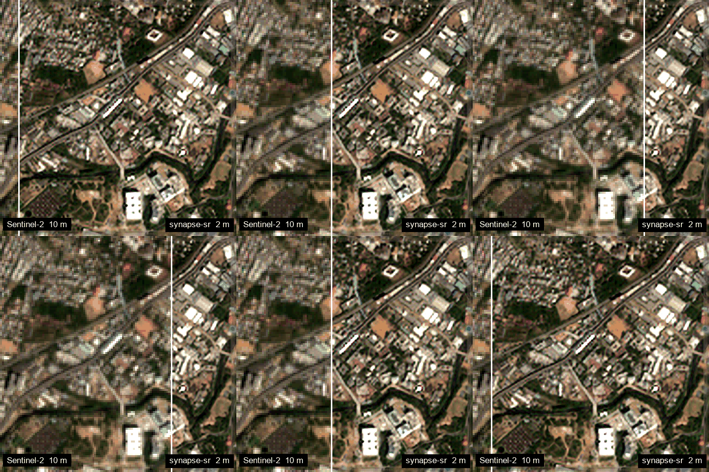 |
Bengaluru city centre · 6 Feb 2025 · 33 / 46 / 21 % 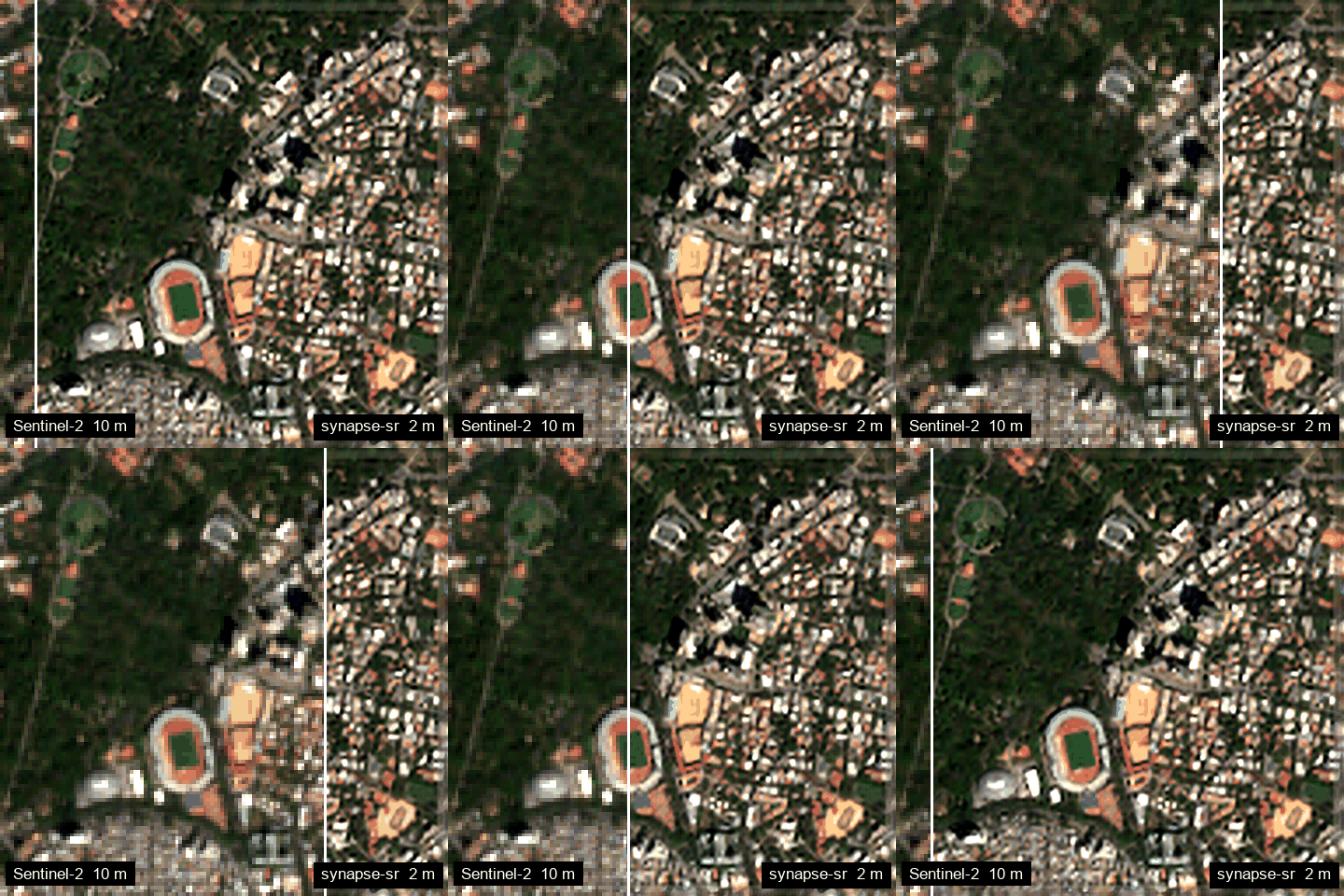 |
Ludhiana, Punjab: fields · 2 Dec 2024 · 40 / 47 / 14 % 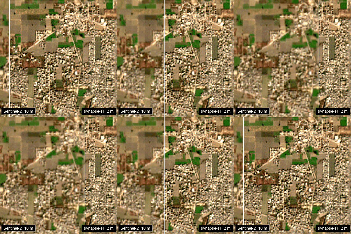 |
Wayanad, Kerala: landslide area · 24 Feb 2025 · 88 / 10 / 1 % 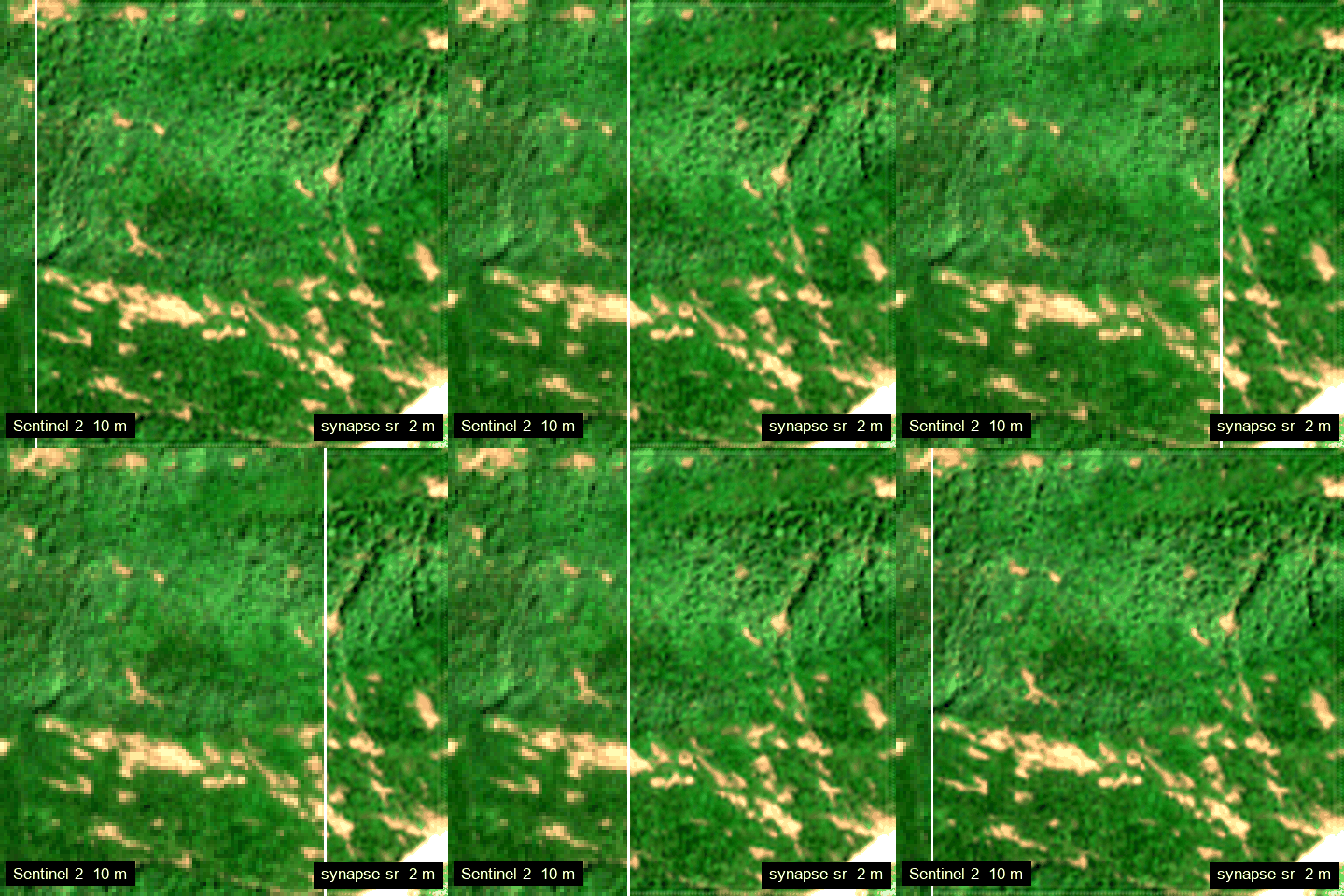 |
Reproduce: pip install "synapse-sr[stac]" pillow, then python tools/make_gifs.py --weights synapse-pro-v2.safetensors --out gifs.
Recipes
Process a whole folder
import synapse_sr

import pathlib
from synapse_sr import Pro

model = Pro.from_pretrained()                        # load once, reuse for every file
out = pathlib.Path("out_2m"); out.mkdir(exist_ok=True)
for tif in sorted(pathlib.Path("scenes").glob("*.tif")):
    if tif.stem.endswith("_scl"):
        continue                                     # cloud masks next to scenes are picked up automatically
    r = model.super_resolve(tif)
    r.save(out / tif.name)
    print(tif.name, r.summary(print_=False)["consistency_rms_over_tau"])
Or from the shell: for f in scenes/*.tif; do synapse-sr "$f" "out_2m/$(basename "$f")"; done.
Only an area of interest from a big scene
Crop at 10 m first. Every 10 m pixel you skip saves 25 output pixels of work. Writing the crop as a small GeoTIFF keeps its coordinates, so the result is georeferenced too.
import rasterio
from rasterio.windows import Window
from synapse_sr import Pro

win = Window(col_off=0, row_off=0, width=64, height=64)          # 640 m x 640 m, in 10 m pixels
with rasterio.open("T43PGQ_full_scene.tif") as src:
    profile = dict(src.profile, width=win.width, height=win.height, transform=src.window_transform(win))
    with rasterio.open("aoi.tif", "w", **profile) as dst:
        dst.write(src.read(window=win))
        dst.descriptions = src.descriptions
        dst.update_tags(**src.tags())                           # keeps BOA_ADD_OFFSET

r = Pro.from_pretrained().super_resolve("aoi.tif")
r.save("aoi_2m.tif")
To select by map coordinates instead, build the window with
rasterio.windows.from_bounds(xmin, ymin, xmax, ymax, src.transform) in the scene's CRS.
A laptop without a GPU
import synapse_sr

from synapse_sr import Flash, Pro

model = Flash.from_pretrained(device="cpu")          # ~1 s per 1.28 km scene on a laptop CPU
# model = Pro.from_pretrained(device="cpu")          # works everywhere; slower on CPU
r = model.super_resolve("scene.tif", batch=1)
Inside Docker or Kubernetes, set OMP_NUM_THREADS to the number of cores you actually have.
Google Earth Engine export
Export the ten bands the model uses, at 10 m, with names, as surface reflectance DN:
var img = ee.ImageCollection("COPERNICUS/S2_SR_HARMONIZED")
  .filterBounds(aoi).filterDate("2025-01-01", "2025-03-15")
  .sort("CLOUDY_PIXEL_PERCENTAGE").first()
  .select(["B4", "B3", "B2", "B8", "B5", "B6", "B7", "B8A", "B11", "B12"]);
Export.image.toDrive({image: img.toUint16(), region: aoi, scale: 10, crs: img.select("B4").projection().crs(),
                      fileFormat: "GeoTIFF", description: "s2_for_synapse"});
from synapse_sr import Pro

r = Pro.from_pretrained().super_resolve("s2_for_synapse.tif",
                                        band_names=["B04", "B03", "B02", "B08", "B05", "B06", "B07", "B8A", "B11", "B12"],
                                        offset=0)          # the HARMONIZED collection already removed the offset
S2_SR_HARMONIZED has the processing-baseline 04.00 offset removed, so pass offset=0. Raw S2_SR scenes after
25 January 2022 need offset=-1000.
xarray, stackstac and cubo
import synapse_sr

import cubo                                          # pip install cubo
from synapse_sr import Pro
da = cubo.create(lat=12.92, lon=77.50, collection="sentinel-2-l2a",
                 bands=["B04", "B03", "B02", "B08", "B05", "B06", "B07", "B8A", "B11", "B12"],
                 start_date="2025-02-01", end_date="2025-02-10", edge_size=128, resolution=10)
r = Pro.from_pretrained().super_resolve(da.isel(time=0))
out = r.to_xarray()                                  # (band, y, x) with 2 m coordinates
An NDVI time series on trusted pixels
import numpy as np, synapse_sr
from synapse_sr import Pro

model = Pro.from_pretrained()
months = [("2024-11-01", "2024-11-30"), ("2024-12-01", "2024-12-31"), ("2025-01-01", "2025-01-31")]
for start, end in months:
    r = model.super_resolve(synapse_sr.fetch_sentinel2(30.935, 75.800, start, end, size_m=1280))
    ndvi = r.indices()["ndvi"]
    print(start, "mean NDVI:", round(float(np.nanmean(ndvi[r.support == 2])), 3))
Restricting statistics to support == 2 keeps prior-dominated pixels out of the numbers.
Per-field statistics with polygons
import synapse_sr

import geopandas as gpd, numpy as np, rasterio.features
from synapse_sr import Pro

r = Pro.from_pretrained().super_resolve("fields.tif")
fields = gpd.read_file("parcels.gpkg").to_crs(r.profile["crs"])
t = r.profile["transform"]
t2 = t * t.scale(1 / 5)                              # the 2 m output grid
ids = rasterio.features.rasterize(zip(fields.geometry, range(1, len(fields) + 1)), out_shape=r.image.shape[1:],
                                  transform=t2)
ndvi, err = r.ndvi(), r.uncertainty()[3]
for i, row in enumerate(fields.itertuples(), 1):
    m = (ids == i) & r.valid
    print(row.Index, "NDVI", round(float(np.nanmean(ndvi[m])), 3), "± NIR error", round(float(err[m].mean()), 4))
Flood extent between two dates
import synapse_sr
from synapse_sr import Pro

model = Pro.from_pretrained()
kw = dict(lat=9.60, lon=76.40, size_m=2000)                  # Kuttanad, Kerala
before = model.super_resolve(synapse_sr.fetch_sentinel2(start="2024-03-01", end="2024-04-30", **kw))
try:
    after_scene = synapse_sr.fetch_sentinel2(start="2024-08-01", end="2024-09-30", max_cloud=60, **kw)
except LookupError as e:                                     # no scene under the cloud limit in that window
    raise SystemExit(f"{e}: widen the dates or raise max_cloud")
after = model.super_resolve(after_scene)
flood = synapse_sr.change(before, after, "ndwi")
print(f"new water: {flood.area_km2:.2f} km2, could not assess: {100 * flood.unreliable_fraction:.0f} %")
- Clouds in the monsoon. Clear scenes are rare during the monsoon. The default
max_cloud=20(percent of the whole tile) found no scene for August to September 2024 here. Raising it is safe, because cloudy pixels are still masked one by one from the scene classification layer. They count towardsunreliable_fraction, not towards the flooded area. - Same grid. Both dates must come out on the same grid.
fetch_sentinel2gives that for a fixed point andsize_m, as long as both scenes come from the same Sentinel-2 tile.
Use the output in QGIS
import synapse_sr
r = synapse_sr.super_resolve("scene.tif")

r.save("scene_2m.tif")                               # bands 1-4: B04 B03 B02 B08; 5-8: ERRSCALE; 9: SUPPORT
In QGIS, set Multiband colour to red = band 1, green = band 2, blue = band 3. Add the file again with band 9 as
Paletted / unique values to see the support classes. Use with_confidence=False if your GIS expects exactly four
bands.
Show a progress bar inside your own application
from synapse_sr import Pro
model = Pro.from_pretrained()

def on_tile(done, total):
    my_progress_widget.set(done / total)

r = model.super_resolve("scene.tif", progress=on_tile)
progress=False silences it; SYNAPSE_SR_QUIET=1 silences it everywhere.