Home


Sentinel-2 at 2 m, with every pixel accounted for.
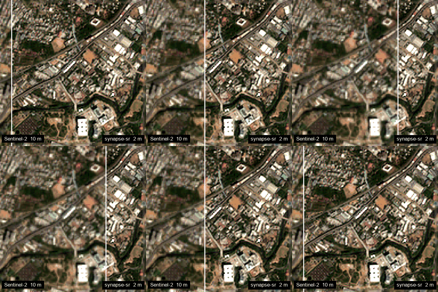
synapse-sr turns a Sentinel-2 L2A scene into a 2.0 m red, green, blue and near-infrared GeoTIFF. A physical model of the instrument pins everything the satellite measured. The network only adds what 10 m pixels cannot show, and every result says which is which.


What you can do with it
-
Crop monitoring
NDVI, SAVI, EVI and red-edge NDRE at 2 m, field-boundary maps, statistics restricted to observation-determined pixels.
r.indices()["ndvi"]·synapse_sr.boundaries(r, "field") -
Urban analysis
Building and road edges, built-up index, per-building detection.
synapse_sr.boundaries(r, "urban")·r.indices()["ndbi"] -
Water and floods
2 m water masks, shoreline strength, flooded area between two dates in km².
synapse_sr.change(before, after, "ndwi") -
Disaster assessment
Burn scars, landslides and debris. Change is flagged only where both dates are trustworthy.
synapse_sr.change(before, after, "nbr")
Worked examples: Applications.
Flash or Pro
| Flash (default) | Pro | |
|---|---|---|
| Network | ~0.6 M-parameter CNN, distilled from Pro | 14.4 M-parameter Mamba state-space model |
| Speed | ~1 s per 1.28 km scene on a laptop CPU | ~5 s per scene on a GPU |
| Runs best on | anything: CPU, laptops, integrated graphics, Apple silicon, ARM, GPU | GPU (Colab, Kaggle, workstations) |
| Guarantees | observation-consistent, support map, calibrated uncertainty | the same |
More: Choosing a model and a device.
Why trust it
| Observation-consistent by construction | x_hat = x_base + P_N(delta): the network's contribution lies in the null space of the Sentinel-2 forward model, so re-observing the output reproduces the measurement. |
| Accountable | per-pixel support (observation-determined versus prior-dominated), calibrated uncertainty, validity mask and a measured round-trip consistency on every result. |
| Geospatially exact | GeoTIFF in, GeoTIFF out, CRS and bounds preserved, direct x5 onto a grid that shares the input origin. |
| Runs anywhere | CUDA, Triton, or pure PyTorch on CPU; live progress bars in terminals and notebooks; fully offline once the weights are local. |